Is the Fix Working Or Is It Just Luck?

For the longest time, the website I was working on for my client had background workers that would crash intermittently and then restart. There seemed to be no pattern to when it would happen. The only thing I knew was that it seemed to be happening about twice a day on average.

Then, one day, after upgrading many of the dependencies, the problem all of a sudden seemed to go away. We went a full two weeks without seeing a single crash.

Did I fix it, or did I just get lucky for two weeks? Whichever way you answer, how certain are you?

If you want to know the answer to both questions, welcome to statistics! We’ll give you just enough to be dangerous.

Why Do I Need to Know This?

“In God we trust. All others must bring data” - Management Consultant W. Edwards Deming

If you’re working at a large FAANG company, the smallest decision, such as making a button larger, needs to be backed up with data. “We’re 99.9% sure that the bigger button increases our sales by 2% or more.” If you’re like us, you’re likely on a small team of devs working with a client.  You’ll be taking on lots of project management responsibilities. Clients are more confident if you can back up your conclusions with data.

You don’t need a PhD. You don’t need to memorize formulas. But you do need to know how to reason under uncertainty and how to simulate. The goal of this blog post series is to give you enough intuition without needing to memorize any formulas.

Statistics In 30 Seconds

1. Take the thing you want to prove.
2. Assume it's not true.
3. Ask: How likely are you to see the results you just observed if, in fact, it's not true?
4. If it’s unlikely, that’s evidence you may be right.

How Statistics Is Like Test Driven Development

1. Take the thing you want to prove: that your code is bug-free
2. Assume it’s not true: write tests that you have verified will fail if the code is broken
3. Once you get those tests passing, ask yourself: how likely is it that the code being tested still has bugs if these tests are green?
4. The lower that likelihood, the higher the confidence you have that your code works.

A passing test suite is not proof that your code is bug-free, just like a nice-looking statistical result is not proof that what you are assuming is actually true. It just gives you more confidence than you had before.

This has all been very abstract, so let’s get into concrete examples, starting with the simplest example.

A Note on the Medium

JavaScript isn’t my first choice for statistical computing. But it’s fast, ubiquitous, and perfectly capable of building intuition through simulation. These examples use JavaScript because that’s what many of us already know, and modern engines are more than fast enough.

Flaky Tests: A Simple but Familiar Case

A test fails \~1 in 6 times. You've seen 8 passing runs in a row.  How confident are you that it has been fixed?

This isn’t the most exciting example from a business perspective, but it serves as a valuable learning tool. It's simple enough to show how statistical thinking works without needing a statistics textbook.

If the test still fails 1 in 6 times, then the probability of it passing 7 times in a row is:

‍

Math.pow(5/6, 7) // ≈ 27.9%

That means there’s still a 27.9% chance the test would pass 7 times in a row just by luck, even if nothing changed. How many successful runs would you need to be 99% confident that it's fixed? Play around with the second argument until you get close to 1%. In this case, you'll see that you need to complete 25 successive passes.

‍

Math.pow(5/6, 25) // ≈ 1.04%

If you haven't worked with stats before, I'm willing to guess that this number, 25, is a higher number of green builds than you expected.

Simulation Helps

Using a simulation here is overkill, but I'm showing how to build a simulation for a simple story problem so that you will know how to use it in the context of something more complicated, such as A/B test results.

Flaky Test Simulation (JS)

‍

function scenario(run_count=7, p=5/6) {
  // This scenario simulates the results if you run 7 successive
  // builds on CI, and it returns back the percentage of those 7
  // builds where the flaky test passes

  let total_passing_builds = 0;
  for (let i=0; i<run_count; i++) {
    if (Math.random() < p) {
      total_passing_builds += 1;
    }
  }

  return total_passing_builds / run_count;
}

function run_trials(options = {}) {
  // The point of a simulation is to take that one scenario listed above
  // and run it over and over again.  Then we can look at the summaries
  // of the results.  In this case we want to find the answer to the question
  // "if we run 7 CI builds without fixing the flaky test, what percentage of
  // the time do all 7 builds pass?"

  const defaults = { trial_count: 100_000, run_count: 7, p: 5/6 };
  const { trial_count, run_count, p } = Object.assign({}, defaults, options);

  let trials_where_all_builds_pass = 0;
  for (let trial=0; trial<trial_count; trial++) {
    if (scenario(run_count, p) === 1) {
      trials_where_all_builds_pass += 1;
    }
  }

  return trials_where_all_builds_pass / trial_count;
}

This might not be clear on the first pass what I’m doing. In this simulation, I’m assuming that I have NOT fixed the flaky test. I’m assuming that the test passes at the same rate as before: 5 times out of 6.

Then I’m simulating what happens if I run the test suite 7 times. Each time I run the test suite 7 times, I’m calling that one trial. I’m counting the percentage of trials where the test passes all 7 times. If you copy and paste the code into your own interactive JavaScript console and then run run_trails(), you’ll get a result close to but not exactly the same as the 27.9%.

My real-world data creates the parameters and assumptions for my simulation.

In the real world, my test was passing 5/6 of the time before I attempted to fix the test. In the real world, I ran my test suite 7 times.

Again, using a simulation, in this case, is overkill, but it shows you the first principles for how to use it in situations where the math gets harder.

Now onto something higher-stakes.

You used to see 5 segfaults/week. Two weeks after a fix, you only saw 8.

Did you improve it?

You don’t know how many “chances” there were for the error to happen, just the number of occurrences. This is why Poisson distributions are ideal for rare events.

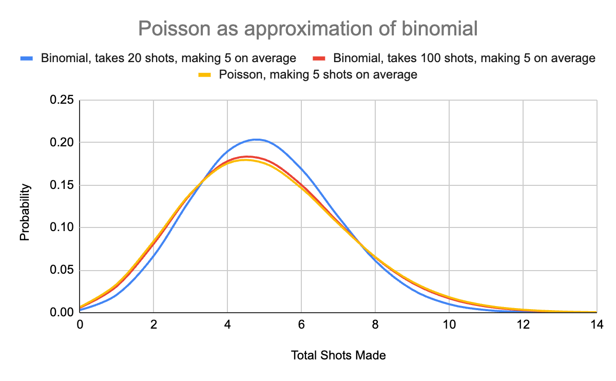
Analogy: Imagine a terrible free-throw shooter:

• Makes 25% of shots, takes 20 → expects 5 hits
• Makes 5% of shots, takes 100 → still 5 hits
• Makes 0.1%, takes 5,000 → still 5 hits

As the denominator grows and the chance per attempt shrinks, the results begin to resemble a Poisson distribution. That’s exactly the shape you get when modeling something like segfaults per trillion CPU cycles. In the graph below, I ignored the free-throw shooter who took 5000 shots and only made 0.1% of them. That line is so close to the Poisson distribution that they look exactly the same on the graph.

Poisson Simulation (JS)

‍

function random_poisson_approximation(expected_number_of_shots_made) {
  // Simulates it with a very large binomial distribution
  const total_shots_taken = Math.floor(expected_number_of_shots_made * 1000);
  const chance_of_making_single_shot = expected_number_of_shots_made / total_shots_taken;

  let total_shots_made = 0;
  for (let i=0; i<total_shots_taken; i++) {
    if (Math.random() < chance_of_making_single_shot) {
      total_shots_made += 1;
    }
  }

  return total_shots_made;
}

function run_trials(options={}) {
  // What we're simulating here is not the number of "free throws" made
  // but the number of errors we've observed.  We assume that the error
  // rate has not changed, that it's still 10 in the observed time period.
  // We then simulate that time period in a single trial/scenario
  // and we find in what percentage we get back 8 or fewer errors

  const defaults = {
    original_average_number_of_errors: 10,
    trial_count: 100_000,
    observed_number_of_errors: 8
  };

  const {
    original_average_number_of_errors,
    trial_count,
    observed_number_of_errors
  } = { ...defaults, ...options };

  // Measures the number of simulated scenarios in which the
  // number of observed errors is 8 or fewer

  let success_count = 0;

  for (let trial=0; trial<trial_count; trial++) {
    let observed_errors_in_scenario = random_poisson_approximation(
      original_average_number_of_errors
    )
    if (observed_errors_in_scenario <= observed_number_of_errors) {
      success_count += 1;
    }
  }

  return success_count / trial_count;
}

So, now that I’ve shown you the formula, let’s go back to the problem that I mentioned earlier. I had a segfault error that was occurring about twice per day. I had gone 2 weeks without an error. If I hadn’t fixed the error, how likely would it be to have gone 2 weeks without an error? If we normally get 2 errors per day, that means 28 errors per two weeks.

‍

run_trials({
  original_average_number_of_errors: 28,
  observed_number_of_errors: 0
})

It’s very likely that if you run this simulation, you’ll get back the number 0. The closed form solution to this question is about 1 in a trillion. Meaning if you run 100,000 trials here, it’s likely NONE of them will show up. So this is an extremely high chance that we have fixed that segfault error.

These two story problems, flaky tests and error rates, are good for engineering teams to talk to each other about. Often, you’ll find it useful to use statistics when talking with a client or product manager. They might be deciding to make a change to the website, and they come to you to help decide whether a new version of the page has better business results for them, which brings us to our final story problem.

A/B Testing: Are You Sure B Is Better?

Imagine your client is deciding between two versions of a page. In one version A of the page, 10 people sign up out of 100 visitors. In another version B, 13 people sign up. How confident are you that version B actually has a higher sign up rate? Was it just dumb luck?

Let’s go back to the fundamentals. Start by assuming the opposite of what you want to prove.

Assume there's no difference between A and B. That means that a total of 200 people visited both pages, and 23 people signed up. That means that the click-through rate for both is 11.5%.

Now you want to ask the question: "How likely is it to see a 30% difference in click-through rate just by random chance?"

Brute Force Simulation (JS)

This is what’s known as a two-sided test. You’re not just checking if B is better than A; you’re checking whether either version performed much better than the other by random chance.

Our example about error rates, on the other hand, is better suited for a one-sided test.  Presumably, you’ve found a portion of the code that could be causing errors. The only question in your mind: is this actually a place where the error is occurring? The only question is: will it reduce the error rate, or not affect it at all?

‍

// Run 10_000 trials
// In each trial, 100 people visit site A and 100 people visit site B
// In the simulation, both sites have the same joint rate
// The final output of each trial will be the click-through rate on page A and the click-through rate on page B

function click_rate(total_visits=100, base_rate=0.115) {
  let click_through_count = 0;
  for (let visit=0; visit<=total_visits; visit++) {
    if (Math.random() < base_rate) {
      click_through_count += 1;
    }
  }

  return click_through_count / total_visits;
}

function percent_difference(rate_a, rate_b) {
  if (rate_a === 0 && rate_b === 0) {
    return 1;
  } else {
    return rate_b / rate_a;
  }
}

function run_trials(options = {}) {
  const DEFAULTS = {
    total_trials: 100_000,
    total_visits: 100,
    base_rate: 0.115,
    target_difference: 1.30,
  };

  const {
    total_trials,
    total_visits,
    base_rate,
    target_difference
  } = { ...DEFAULTS, ...options};

  let success_count = 0;
  for (let trial=0; trial<total_trials; trial++) {
    // Remember we're assuming that there's NO difference between
    // the click through rates on both versions
    let click_rate_a = click_rate(total_visits, base_rate);
    let click_rate_b = click_rate(total_visits, base_rate);

    // Remember this is a two sided test
    // We want to see how likely it is that EITHER page has a click
    // through rate that's at least 30% higher than the other
    let ratio_left  = percent_difference(click_rate_a, click_rate_b);
    let ratio_right = percent_difference(click_rate_b, click_rate_a);
    if (ratio_left > target_difference || ratio_right > target_difference) {
      success_count += 1;
    }
  }

  return success_count / total_trials;
}

Simulation vs Statistics

Each step of the simulation I set up is relatively straightforward. When using the simulation for flaky tests, it was overkill. The flaky test and error rate problems both have simple formulas which give you the answer. In the appendix I’ll show you the math behind A/B testing, and it’ll be clear why writing a simulation can be easier if you haven’t taken a stats course.

Simulations aren’t cheating. They’re how professionals check their math.

Takeaways

• Simulations build intuition.
• When you can’t remember the formula, write the code.
• Confidence isn’t binary. It’s about “how unlikely is what I just saw if nothing changed?”

When in doubt, simulate.

Appendix: The Math Behind the Intuition

In this blog post we explored real-world engineering problems: flaky tests, intermittent errors, A/B testing, and how simulation can help us reason under uncertainty. But what are the mathematical ideas behind these simulations?

This post walks through the core concepts we hinted at during the talk: the distributions, the theorems, and the structural logic of statistical inference. Think of this as the math that powers the intuitions. Here's a quick review:

The Logic of Statistical Inference

To recap, at the heart of statistics is this loop:

1. Take the thing you want to prove.
2. Assume it's not true.
3. Ask: if it's not true, how likely are the results I observed?
4. If they're unlikely, that's evidence that you might be right.

This is the statistical version of test-driven development: assume the code is broken, then test. The more tests that pass, the more confidence you gain — never absolute certainty, but enough to act. Here are some bonus concepts:

Cumulative Distribution Function (CDF)

Many statistical tools use inequalities instead of exact values. For instance:

How likely is it that I flip exactly 496 heads in 1000 fair coin flips? ≈ 2.4%  

How likely is it that I flip 496 or fewer? ≈ 41%

Exact matches are rare. We usually care about whether results are as extreme or more than what we saw. This is where the CDF comes in.

Central Limit Theorem

As you collect more independent samples, their average tends to form a bell curve, the normal distribution, regardless of the shape of the original data.

That’s the central limit theorem in action. It’s why we can often approximate binomial or Poisson processes with a normal distribution, especially with large data.

A Galton Board, which is similar to the game Plinko from the TV show The Price is Right, demonstrates this phenomenon.

Normal distribution has just two parameters:

• ‍Mean (average): where the curve is centered‍
• Standard deviation: how wide or narrow the curve is

Variance of the Mean

Suppose every day you take 50 free throws. How much does your daily average vary? Now imagine that you take 1000 free throws. How much does your daily average vary?  Would it be by more or less than if you only took 50 free throws per day?  (Answer: less)

The more data in each batch, the more stable your averages. This idea is behind confidence intervals: averages from small samples bounce around more than those from large samples.

In A/B testing, this tells us how much variation to expect across different groups and how sure we can be that an observed difference is real.

To get a sense of the variance of the mean, run the same simulation multiple times. See how much the result jumps around.

Parameter Sensitivity: What Simulations Teach Us

One of the best ways to build statistical intuition is to tweak the knobs yourself. When you run simulations, adjusting different parameters reveals how statistical confidence behaves in practice.

Here are four key observations:

1. More Page Visits per Trial → Smaller p-value

Increasing the sample size sharpens your conclusions. The more visits you collect, the easier it is to detect small differences.

2. More Trials → More Stable Estimates

This is key here: more trials don’t mean more real-world data. It means you run more trials based on the SAME real-world data. Running more simulation trials doesn't change the expected result, but it smooths out noise. This is the law of large numbers (aka the law of average): as trials accumulate, estimates converge.

3. Larger Differences → Fewer Samples Needed

A 30% difference is easier to detect than a 3% one. The more dramatic the effect size, the faster you can be confident it's real.

4. Low Overall Rates → Slower Confidence

In the A/B testing example, if both A and B have very low conversion rates (e.g., 0.5%), random fluctuation dominates. You’ll need more data to tell the signal from noise. In this case what matters is the number of people who signed up, not the number of people who visited the page.

Simulation isn't just for getting answers; it’s a learning tool. You see how math responds to real-world conditions, without needing to memorize statistical formulas.

When in Doubt, Simulate

The math can be heavy. Simulations don’t replace understanding, but they let you check your reasoning. They help you internalize probabilities and think statistically without memorizing every formula. I created a gist that demonstrates the math to tie these concepts together.

Now that you've seen what the math looks like, the simulation is a lot easier to grasp. A developer might code the simulation the wrong way, but mathematicians make errors all the time, too.